There is a question that has been bugging me since the first time I read the original Denoising Diffusion Probabilistic Models paper. The setup is elegant: take an image, gradually add Gaussian noise until it is indistinguishable from random pixels, then train a network to undo that process one tiny step at a time. Sampling new images is just running the noise removal in reverse from a fresh patch of randomness. Done.
The question is whether it actually works the way the paper claims, on hardware I can run, with code I have written myself. In particular: does a small diffusion model trained on a few hundred images really produce novel samples that recombine training features in interesting ways, or does it just memorize and slightly perturb?
So I implemented a small pixel-space DDPM, trained it on 64 by 64 emoji faces for 2000 epochs, and saved a 10-image sample grid every 50 epochs. The result is a video of training I can scrub through. The progression from pure noise to coherent (and increasingly weird) emoji faces is the most fun training run I have produced, and the answer to my original question is yes: by epoch 600 the model is already generating combinations of features that do not exist in any training image. That is the part this post is about.
What diffusion actually is, before any equations
Imagine a clean image as a single point in a very high-dimensional space (for a 64x64 RGB image, that is a point in R^12,288). Real images live on some low-dimensional manifold inside that space (most pixel arrangements are not faces, or cats, or anything; the ones that are sit on a tiny structured surface).
Now imagine a process that takes that point and starts walking it around the space by adding small amounts of Gaussian noise at every step. After a few hundred steps, the point has drifted so far from the original manifold that we cannot tell it apart from any other random point. The image is gone. We have pure noise.
The training objective for diffusion is to learn the reverse of this walk. Given a noisy point and a timestep telling us how far along the walk we are, predict the noise that was added at this step so we can subtract it and move one step back toward the data manifold.
If the network learns this reverse step well, sampling becomes mechanical: start at a random point in pixel space (pure noise), apply the learned reverse step a few hundred times, and we arrive somewhere on the data manifold. A new face. Possibly one that does not exist in the training set.
That is the entire idea. The math just makes it precise enough to compute.
The forward process: noise on a schedule
The forward (noising) process is fixed. We do not learn it. It is a Markov chain that adds Gaussian noise at every step:
q(x_t | x_{t-1}) = N(x_t; sqrt(1 - β_t) * x_{t-1}, β_t * I)
The schedule is a sequence of small positive numbers β_1, β_2, ..., β_T that controls how much noise gets added at each step. I used a linear schedule from β_1 = 1e-4 to β_T = 2e-2 over T = 200 steps. Small at the beginning (so we do not destroy the image structure too fast), bigger toward the end (so we end up in a roughly isotropic Gaussian).
The clever piece is that we never need to actually walk the chain step by step during training. There is a closed-form expression that lets us jump from x_0 to x_t in one shot:
x_t = sqrt(alpha_bar_t) * x_0 + sqrt(1 - alpha_bar_t) * epsilon
where epsilon ~ N(0, I), alpha_t = 1 - β_t, and alpha_bar_t = product of all alpha_s for s = 1 to t (the cumulative product). This drops out of the algebra of composing Gaussian-on-Gaussian transitions, and it is the single most important simplification in the whole setup. We can sample any noisy version of any image instantly:
def q_sample(self, x0, t, noise=None):
    # Jump directly to timestep t in one shot
    if noise is None:
        noise = torch.randn_like(x0)

    sqrt_alpha_bar_t        = self.sqrt_alpha_bars[t].view(-1, 1, 1, 1)
    sqrt_one_minus_alpha_bar_t = self.sqrt_one_minus_alpha_bars[t].view(-1, 1, 1, 1)

    xt = sqrt_alpha_bar_t * x0 + sqrt_one_minus_alpha_bar_t * noise
    return xt, noise
This means each batch during training can teach the model many timesteps at once. We sample a random t for every image in the batch, noise each image to that level in one operation, and the model has to handle all of them.
The training objective: predict the noise
This is the part that reads like sleight of hand the first time. The standard derivation says the variational lower bound on the log-likelihood, when simplified, becomes a weighted MSE between the actual noise we added and what the network predicts. The weighting is dropped in practice because the unweighted version trains more stably. So the loss collapses to:
L = E_{x_0, t, epsilon} [ || epsilon - epsilon_theta(x_t, t) ||^2 ]
In English: sample a clean image, sample a timestep, sample some noise, build the noisy image, ask the model what noise was added, compute MSE.
def forward(self, x0):
    b = x0.shape[0]
    t = torch.randint(0, self.T, (b,), device=x0.device, dtype=torch.long)

    xt, noise = self.q_sample(x0, t)

    pred_noise = self.eps_model(xt, t)
    return F.mse_loss(pred_noise, noise)
That is the entire training step. Twelve lines including the comments. The simplicity is what makes diffusion so different from GANs (with their adversarial dance) or autoregressive models (with their token-by-token loss). One MSE.
The reason we predict the noise rather than the clean image is mostly empirical. Both are equivalent reparameterizations: knowing x_t, t, and either x_0 or epsilon lets us recover the other. But predicting epsilon works much better in practice. The intuition I have settled on is that noise has roughly the same scale at every timestep (it is always a unit Gaussian), while x_0 would have to be predicted from very different information at different t values. Predicting noise gives the model a more uniform target across the entire training distribution.
The denoiser: a U-Net with time conditioning
The network that predicts the noise (epsilon_theta) is a U-Net. The U-Net architecture is dominant in diffusion for one specific reason: noise removal needs to operate at multiple spatial scales. A few-pixel-wide noise pattern needs to be cleaned up by a different mechanism than a full-image-scale color shift. The U-Net’s encoder/decoder structure with skip connections lets the network see the input at every resolution and combine those views in the output.
class UNet(nn.Module):
    def __init__(self, c_in=3, c_out=3, time_dim=256, base=96):
        super().__init__()
        b = base
        self.time = SinusoidalTimeEmbedding(time_dim)

        # Encoder (down)
        self.inc   = ResidualBlock(c_in, b)
        self.down1 = Down(b, b * 2, time_dim)
        self.down2 = Down(b * 2, b * 4, time_dim)
        self.attn1 = SelfAttention(b * 4)
        self.down3 = Down(b * 4, b * 4, time_dim)

        # Bottleneck
        self.bot1 = ResidualBlock(b * 4, b * 8)
        self.bot2 = ResidualBlock(b * 8, b * 8, residual=True)
        self.bot3 = ResidualBlock(b * 8, b * 4)

        # Decoder (up), with skip connections
        self.up1 = Up(b * 4, b * 4, b * 2, time_dim)
        self.attn2 = SelfAttention(b * 2)
        self.up2 = Up(b * 2, b * 2, b, time_dim)
        self.up3 = Up(b, b, b, time_dim)

        self.out = nn.Conv2d(b, c_out, 1)

    def forward(self, x, t):
        t = self.time(t)               # sinusoidal time embedding
        x1 = self.inc(x)
        x2 = self.down1(x1, t)
        x3 = self.attn1(self.down2(x2, t))
        x4 = self.down3(x3, t)
        x4 = self.bot3(self.bot2(self.bot1(x4)))
        x  = self.attn2(self.up1(x4, x3, t))
        x  = self.up2(x, x2, t)
        x  = self.up3(x, x1, t)
        return self.out(x)
Three details inside this are worth slowing down on.
Sinusoidal time embeddings. The model needs to know what timestep it is operating on, because the right denoising behavior at t=199 (mostly noise) is very different from t=10 (almost clean). We could pass t as a single integer, but neural networks generally do not like raw integers as input. The standard trick (borrowed from the Transformer paper) is to expand t into a higher-dimensional vector using sines and cosines at exponentially-spaced frequencies. This gives the network a smooth, structured representation of where it is in the diffusion process.
Time embedding injected at every layer. The Down and Up blocks each have their own learned linear projection of the time embedding, and they add it to the spatial feature map after the convolutional operations. The network is constantly being reminded which timestep it is at, and different layers can learn to use that information differently.
Self-attention at certain resolutions. The U-Net has self-attention layers at the deeper feature maps. This is essential for getting global structure right. Convolutions only see local neighborhoods, but a face has long-range structural constraints (the two eyes need to be roughly symmetric, the mouth needs to be below the eyes). Self-attention lets the network reason about distant pixels, which is the difference between “blurry collection of features” and “coherent face.”
The full denoiser has a few million parameters. Small by modern standards.
Sampling: walking the noise back to an image
Once the noise predictor is trained, sampling is a loop. Start with pure noise, predict the noise that “must have been added” to get there, subtract a scaled version of it, add a tiny bit of fresh noise (except on the very last step), repeat:
@torch.no_grad()
def p_sample(self, xt, t_scalar, model):
    b = xt.shape[0]
    t = torch.full((b,), t_scalar, device=xt.device, dtype=torch.long)

    # The trained noise predictor
    eps_theta = model(xt, t)

    beta_t                       = self.betas[t].view(-1, 1, 1, 1)
    sqrt_recip_alpha_t           = self.sqrt_recip_alphas[t].view(-1, 1, 1, 1)
    sqrt_one_minus_alpha_bar_t   = self.sqrt_one_minus_alpha_bars[t].view(-1, 1, 1, 1)

    # Mean of p(x_{t-1} | x_t), from the DDPM derivation
    model_mean = sqrt_recip_alpha_t * (
        xt - (beta_t / sqrt_one_minus_alpha_bar_t) * eps_theta
    )

    # Final step: no noise, just the mean
    if t_scalar == 0:
        return model_mean

    # Earlier steps: add a stochastic term sampled from the posterior variance
    posterior_var_t = self.posterior_variance[t].view(-1, 1, 1, 1)
    noise = torch.randn_like(xt)
    return model_mean + torch.sqrt(posterior_var_t) * noise

@torch.no_grad()
def sample(self, n, model):
    x = torch.randn(n, CHANNELS, IMAGE_SIZE, IMAGE_SIZE, device=self.betas.device)
    for t in reversed(range(self.T)):
        x = self.p_sample(x, t, model)
    return x
That is 200 forward passes through the U-Net per generated image, which is one of the things that makes diffusion slow at inference compared to GANs. Newer techniques (DDIM, consistency models, distillation) reduce this to a few or even a single step. The basic DDPM keeps all 200 because the math is cleanest that way and it makes the training-inference relationship transparent.
Watching the model learn
Training ran for 2000 epochs on roughly 200 emoji face images. The loop saved a 10-image sample grid every 50 epochs, generated using the EMA-smoothed copy of the network for stability. What it looks like over time is the most useful result.
At epoch 50, after about 10,000 batches, the model is barely doing anything:
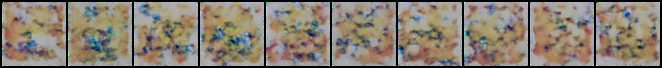
Each sample is a 64x64 patch of color noise. We can squint and see that some of the warm-tone clusters are roughly round. The model has learned that “emoji” usually means “warm-colored circle on a lighter background,” but nothing more. The training loss at this point is still dropping rapidly.
By epoch 200, the model has noticed that emojis have facial features. The proportions are wrong, the colors are wrong, but there are unmistakable mouth-like horizontal bars and eye-like dark spots:
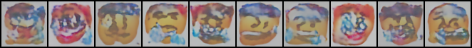
These look like face emoji ghosts. We can see the mustache on a few of them, faint suggestions of teeth, the general “round head with darker features in the middle” arrangement. None of them are individual recognizable emojis yet. They look like the model is averaging over many faces and producing the mean.
By epoch 600, the model has crystallized:

These are recognizable emojis. We can name what most of them are. Two cowboy faces, a sweat-drop face, a smiling face, a face with circles for cheeks, a vomit face, two more smiling faces, a sweat-drop face. The colors are right. The features are crisp. There are still small artifacts (the cowboy hat on the second image is slightly malformed), but at this point the model is clearly producing emoji-shaped things from pure noise.
Importantly, several of these are not exact copies of training images. The cowboy hat plus sweat drop combination, for example, is something the model is recombining. We will come back to this.
By epoch 1200, the quality has improved further:

The crying face on the left has clean tear streams. The third face has a cowboy hat that is clearly drawn. The angry-with-symbols face on the right (the censored-cursing emoji) has visible glyph-like marks where the mouth should be. The second face has a stuck-out tongue overlaid on a sweating face, which is itself a Mr. Potato Head combination because no single training image has both.
By epoch 2000, the model has more or less converged:

The samples are sharp. The features are clean. We have angry-with-symbols faces, sweat faces, clown faces (with the painted nose visible), and one angel face with the halo at the top. None of these are pixel-perfect copies of training samples. The model is clearly composing.
The Mr. Potato Head effect
This is the part of the experiment I cared most about, and the part the assignment writeup focused on too.
The hypothesis going in was that a diffusion model trained on a small set of distinct face categories would learn to recombine features across categories, rather than memorizing the categories themselves. If that hypothesis is right, we should see novel face emojis that mix features from different training emojis: a halo from one, a tongue from another, a hat from a third, all on the same face.
And we do. Looking at samples saved across epochs:
-
Epoch 600 produced a smiling face with both a cowboy hat (a feature from the cowboy emoji) and a single tear (a feature from the sad emoji) and a stuck-out tongue (a feature from the silly emoji). Three features fused on one face. No training image has this combination.
-
Epoch 850 produced a sweating face with glasses. The glasses come from the nerd emoji, the sweat from the embarrassed emoji. The result is neither.
-
Epoch 1200 produced a face with the upper-blue-forehead from the cold emoji, the red flush from the angry emoji, and tears on both sides from the crying emoji. A three-feature combination.
-
Epoch 1350 produced a face with both an angel halo and a stuck-out tongue. An angel-emoji feature on a silly-emoji body.
-
Epoch 1600 produced a face with a birthday cap (party emoji), a dollar-sign mouth (money emoji), and neutral dot eyes (a different category entirely).
This pattern is consistent across the training run. Some emoji faces are essentially cleaner copies of training samples. Most of the interesting ones are clean combinations of features from multiple training categories. The model learned that emojis have hats, eyes, mouth shapes, color tones, and tear patterns as compositional features it can mix and match, rather than learning that emojis come in fixed categories like cowboy or angel or sweating.
This is the property that makes diffusion models genuinely generative rather than recall machines. If the model were memorizing, every sample would resemble exactly one training image. Instead, it has implicitly learned a structured representation where faces can be decomposed into and recomposed from a set of attribute-like features. Sampling pulls one combination out of that combinatorial space.
What this whole thing taught me
The first instinct from this experiment is about how short the math actually is. The DDPM derivation looks intimidating in the original paper because it leans on variational inference and probability theory. But the operational summary is genuinely tiny: forward process is x_t = sqrt(alpha_bar_t) * x_0 + sqrt(1 - alpha_bar_t) * epsilon, the loss is MSE between predicted and true epsilon, the sampling step is x_{t-1} = (1/sqrt(alpha_t)) * (x_t - (beta_t / sqrt(1 - alpha_bar_t)) * epsilon_theta) + noise. Three equations. The whole rest of the implementation is bookkeeping (precomputing constants, handling batches, building a U-Net).
The second instinct is about how training looks. Diffusion training is the most well-behaved thing I have run. The loss curve drops smoothly. There is no GAN-style instability, no mode collapse, no need for fancy tricks. Adam at 1e-5 to 1e-4, batch 64, EMA on the parameters for sample stability, train until our patience runs out. The model just gets better.
The third instinct is the most useful one. The Mr. Potato Head combinations are the visible evidence of something the literature talks about but that is hard to feel without watching it happen: diffusion models learn factorized representations of their data. They do not memorize images. They learn the underlying axes of variation (color, expression, accessories) and can interpolate or recombine along those axes when sampling. This is the same property that lets larger diffusion models generate “an astronaut riding a horse in the style of Van Gogh.” It is just the small version. The model has never seen an astronaut riding a horse, and it has never seen a face emoji with a halo plus a tongue, but in both cases the generative process is the same: pull one combination out of a learned compositional space.
The fourth instinct is more practical. Watching training happen is severely underrated as a debugging tool. The fact that I saved a sample grid every 50 epochs and could scrub through them like a video taught me more about the model’s behavior than any numerical metric. By epoch 200 I knew the U-Net was learning something. By epoch 600 I knew it had crossed a quality threshold. By epoch 1200 I knew the Mr. Potato Head effect was real. Without the visual log, all I would have seen was a smoothly declining loss curve and a single sample grid at the end. The qualitative trajectory of training is itself a piece of evidence about whether the model is doing what we think it is doing.