A tiny neural network and four experiments I ran on it

I have used model.fit(x, y) more times than I can count. Most of the time it works. Sometimes the loss does not go down and I poke at the learning rate or the architecture or the data until it does. The poking has been pattern matching more than understanding. So one weekend I decided to actually slow down and build a tiny neural network from scratch, then run a few experiments on it that I knew would teach me something I had been nodding along to for years.

The system is small on purpose. Two input features, one hidden layer, two output classes. Four little 2D datasets to train on. The whole thing fits on one screen. The point is not the model. The point is being able to watch every choice we make show up as a visible change in the output, instead of disappearing into a framework abstraction.

Four experiments came out of this:

1. How big does the hidden layer need to be, and what changes when we get it wrong?
2. What actually happens if we use MSE loss for binary classification instead of cross-entropy?
3. Can we reproduce the whole pipeline in raw NumPy, with backprop derived by hand?
4. What if we add a regularization term that pushes the hidden units to learn different features?

Each one taught me something I now find myself using when I read papers or talk to ML engineers. This post walks through all four with the actual code I wrote, the actual outputs I saw, and the parts of the math that became permanent only after I watched them on screen.

The setup

Before the experiments, the chassis. The model is a 2-layer multi-layer perceptron with k hidden units, tanh activation, and a softmax (or sigmoid, in one experiment) output. In PyTorch that is three lines:

model = nn.Sequential(
    nn.Linear(2, k),
    nn.Tanh(),
    nn.Linear(k, 2),
)

The four datasets are 2D scatter problems with binary labels: two_gaussians (linearly separable, two blobs), xor (the classic four-quadrant problem), center_surround (one circle inside another), and spiral (two interleaved arms). They were chosen to span a range of geometric difficulty. A logistic regression solves the first one. The last one needs an actual nonlinear decision boundary.

I trained on each dataset with vanilla SGD at learning rate 0.5, normalized the features using training-set statistics, and used a held-out validation split with early stopping (patience 50) to pick the best checkpoint. Standard hygiene. Nothing fancy. The interest is in what changes when we vary the things we are about to vary.

Experiment 1: how big should the hidden layer be?

The textbook answer is “small enough not to overfit, large enough not to underfit, find the sweet spot on validation.” Fine. But what does that actually look like when we have to pick a number?

I swept k over [2, 3, 5, 7, 9] for each dataset and recorded the lowest validation loss reached:

Two things jump out. First, on two_gaussians, all five values are basically the same. The dataset is linearly separable, so two hidden units have plenty of capacity. Adding seven more does not help, because there is nothing left to learn. This is a useful negative result: bigger is not better when the data does not need it.

Second, on xor, going from k=2 to k=3 cuts the loss in half. From k=3 to k=5 it cuts in half again. After that, gains taper. This is the shape of a model finally having enough capacity to bend the decision boundary. Until k=3, the network literally cannot represent the XOR function with two hidden tanh units. With k=3 it can, just barely. With k=5 it can do so comfortably.

The spiral story is the most dramatic. With k=2 it gives up: 60 percent accuracy is barely better than chance for a balanced binary problem. The decision boundary cannot bend enough. By k=9 it is nailing the test set perfectly:

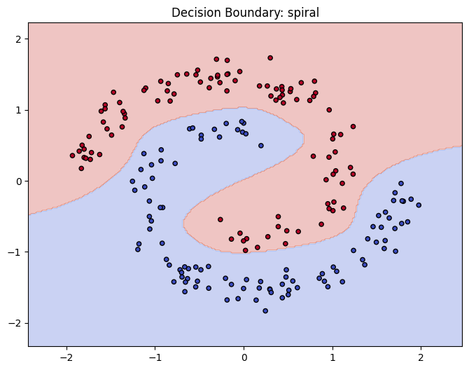
The relevant code is the inner part of the training loop, which is just SGD with early stopping:

for epoch in range(1000):
    model.train()
    optimizer.zero_grad()
    loss = criterion(model(train_features), train_targets)
    loss.backward()
    optimizer.step()
 
    model.eval()
    with torch.no_grad():
        val_loss = criterion(model(val_features), val_targets)
 
    if val_loss < min_val_loss:
        min_val_loss = val_loss
        best_state = model.state_dict().copy()
        patience_counter = 0
    else:
        patience_counter += 1
 
    if patience_counter >= 50:
        break

I settled on k=9 as the value that worked across all four datasets. Not because nine is magic, but because nine was the smallest number where additional capacity stopped lowering validation loss. That is the actual rule, written down: pick the smallest hidden width that no longer underfits, judged on a held-out set. Anything bigger is paying for parameters we are not using.

The deeper instinct that came out of this is that we should stop talking about “the right hidden layer size” in the abstract. The right size is a function of the dataset’s geometric complexity, and it is empirical. The conversation worth having is “how curvy does the decision boundary need to be,” not “is k=64 enough.” The first one has an answer. The second one does not.

Experiment 2: what if we use MSE instead of cross-entropy?

The convention is to use cross-entropy for classification and MSE for regression. I knew the convention. I had never tested what happens when we ignore it.

For experiment 2, I kept everything the same as experiment 1 but swapped the loss. The output layer goes from a 2-unit softmax to a 1-unit sigmoid (predictions in 0 to 1, treated as a regression target):

model = nn.Sequential(
    nn.Linear(2, k),
    nn.Tanh(),
    nn.Linear(k, 1),
    nn.Sigmoid(),     # output in (0, 1)
)
optimizer = optim.SGD(model.parameters(), lr=0.5)
criterion = nn.MSELoss()

The targets become floats (0.0 or 1.0). The training loop is the same. The accuracy at the end of training is the same, give or take a percent.

The thing that is not the same is the number of epochs we need to get there. Cross-entropy from experiment 1 was happy with 1000 epochs and patience 50. MSE needed me to bump those to 2000 epochs and patience 100, otherwise it would early-stop before it had really converged.

The reason is not subtle once we work through the gradient. With MSE on a sigmoid output, the gradient of the loss with respect to the pre-activation z is:

∂L/∂z = (σ(z) - t) · σ'(z)
       = (σ(z) - t) · σ(z) · (1 - σ(z))

The first factor is the error: how far off our prediction is from the target. The second factor, σ'(z) = σ(z)(1 - σ(z)), is the derivative of the sigmoid. And here is the issue. When σ(z) is close to 0 or 1, that derivative is close to zero. So when the model is confidently wrong (σ(z) = 0.99 for a target of 0, say), the gradient signal collapses. The optimizer wants to push hard. The math hands it back almost nothing. Training crawls.

Cross-entropy paired with sigmoid does not have this problem. The gradient of the binary cross-entropy loss L = -t log σ(z) - (1 - t) log(1 - σ(z)) with respect to z works out to:

∂L/∂z = σ(z) - t

The σ'(z) factor that hurts us in the MSE case cancels out cleanly. We are left with just the prediction-minus-target error. The signal stays strong even when the model is saturated. We get a strong push when we are wrong, regardless of how confidently wrong we were.

That cancellation is the entire reason for the convention. It is not a stylistic preference. It is not “cross-entropy is more theoretically motivated for classification” (though that is also true). It is a statement about how the loss interacts with the activation, and which combination keeps gradients flowing. MSE on a sigmoid output is mathematically valid. It is also practically slow.

I had read this exact paragraph in textbooks. Watching the loss curves diverge, with MSE plateauing while cross-entropy was already converged, made it permanent.

Experiment 3: building the whole thing in NumPy

Experiment 3 was the one I was avoiding. The professor in me knew it was the most useful exercise. The engineer in me knew how unpleasant it would be. I wrote it anyway.

The forward pass is unremarkable. Linear, tanh, linear, softmax:

def compute_softmax(z):
    # Numerical stability: shift by max before exp
    z_shifted = z - np.max(z, axis=1, keepdims=True)
    exp_z = np.exp(z_shifted)
    return exp_z / np.sum(exp_z, axis=1, keepdims=True)
 
def forward(x, W1, b1, W2, b2):
    z1 = x @ W1 + b1          # pre-activation, layer 1
    h  = np.tanh(z1)          # hidden activation
    z2 = h @ W2 + b2          # pre-activation, layer 2
    y  = compute_softmax(z2)  # output probabilities
    return y, h, z1

The interesting part is the backward pass through softmax-then-cross-entropy. If we differentiate them separately, both are unpleasant. Softmax has a Jacobian where each output depends on every input (because of the normalizing denominator across classes). Cross-entropy has a sum over classes with logarithms inside it. The chain rule between them produces a wall of subscripts that is genuinely hard to keep straight.

Compose them, though, and almost everything cancels.

The cross-entropy loss for one example with one-hot target t and predicted probability vector y = softmax(z) is:

L = -Σᵢ tᵢ log yᵢ

The gradient of L with respect to the pre-softmax logits z is:

∂L/∂z = y - t

That is it. Predicted probabilities minus the one-hot target. Same shape as z. No Jacobians. No leftover terms. (The full derivation needs about a page of careful index work, then the cross-terms collapse.)

Once we have ∂L/∂z, the rest of backprop is straightforward chain rule:

def backward(x, target_onehot, y, h, W2):
    n = x.shape[0]
    # The clean cancellation: ∂L/∂z2 = (y - t) / batch_size
    dz2 = (y - target_onehot) / n
 
    dW2 = h.T @ dz2
    db2 = np.sum(dz2, axis=0)
 
    # Backprop through tanh: derivative is (1 - h^2)
    dz1 = (dz2 @ W2.T) * (1 - h ** 2)
    dW1 = x.T @ dz1
    db1 = np.sum(dz1, axis=0)
 
    return dW1, db1, dW2, db2

To check that the manual gradients match what PyTorch’s autograd would compute, I ran the same input through both:

# Run a small batch through PyTorch
x_torch = torch.tensor(x_scaled[:10], dtype=torch.float32)
y_torch = torch.tensor(y_raw[:10], dtype=torch.long)
torch.nn.CrossEntropyLoss()(ref_net(x_torch), y_torch).backward()
 
# Same batch through my NumPy code
preds, hidden, _ = forward(x_scaled[:10], W1, b1, W2, b2)
dW1_manual, _, _, _ = backward(x_scaled[:10], one_hot[:10], preds, hidden, W2)
 
# Maximum elementwise difference
diff = np.abs(dW1_manual.T - ref_net[0].weight.grad.numpy()).max()
print(f"Grad check: max difference = {diff:.2e}")
# Grad check: max difference = 5.96e-08

A difference of 5.96e-08 is just floating-point noise. The math is the same.

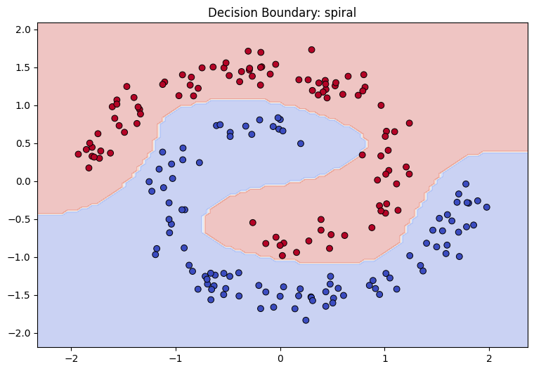
I trained this from-scratch implementation on all four datasets and got accuracies that matched the PyTorch version of experiment 1 to within a percentage point: 91.5 percent on two_gaussians, 97.5 on xor, 75.5 on center_surround, and 100 on spiral. The decision boundary on the spiral, drawn from probabilities that came out of my own backprop, looked like this:

There is a small product lesson tucked into all of this. PyTorch ships a single op called torch.nn.functional.cross_entropy that takes raw logits (skipping softmax entirely) and computes the loss in one numerically stable expression. It is not bundled for convenience. It is bundled because the gradient is cleaner when we treat softmax and cross-entropy as a unit, and because computing them separately is both slower and prone to overflow when logits are large. APIs that look merged for taste sometimes have real reasons underneath. The way we figure out which is which is by deriving them.

The other lesson is more practical. There is a specific kind of confidence I now have when I read a paper that says “we use cross-entropy loss with softmax output.” Before this exercise, that sentence was a fact to absorb. After this exercise, that sentence describes a choice with mathematical structure I have personally verified. The two confidences feel completely different.

Experiment 4: a regularization term that pushes the model harder

The first three experiments were about the basic mechanics. Experiment 4 was the one I was actually curious about. What happens if we deliberately constrain the network in a useful way, by adding a term to the loss that says “your hidden units should learn different features from each other”?

The standard tool is an orthogonality penalty. We take the first-layer weight matrix W (one row per hidden unit), compute W Wᵀ (a Gram matrix of inner products between rows), and penalize the off-diagonal entries. A perfectly orthogonal weight matrix has a diagonal Gram matrix. Anything off-diagonal is two hidden units pointing in similar directions, which is wasted capacity.

def compute_ortho_penalty(net):
    W = net[0].weight                 # (hidden_units, input_dim)
    gram = W @ W.t()                  # pairwise inner products
    diag = torch.diag(torch.diag(gram))
    off_diagonal = gram - diag
    return torch.sum(off_diagonal ** 2)

We add this to the standard loss with a weight λ:

total_loss = ce_loss(predictions, targets) + λ * compute_ortho_penalty(model)

I ran the spiral dataset with k=3 (small capacity, on purpose, so the regularizer has something to fight over) and tried two values of λ.

With λ = 1, the regularizer dominated the gradient. The hidden units stayed almost orthogonal, which is what we asked for. They were also almost useless, because the cross-entropy term could not move them toward solving the actual problem. Accuracy collapsed.

With λ = 0.01, things worked beautifully. Test accuracy went from 84 percent (no regularization) to 88.5 percent. The model fit the spiral better than it had without the term, because the regularizer gently encouraged each hidden unit to specialize on a different region of the input space instead of duplicating each other’s work.

The most fun part of this experiment was visualizing what each hidden unit had actually learned. With only three hidden units, we can plot each one’s individual decision surface (the boundary where its tanh activation crosses zero) alongside the composite output:

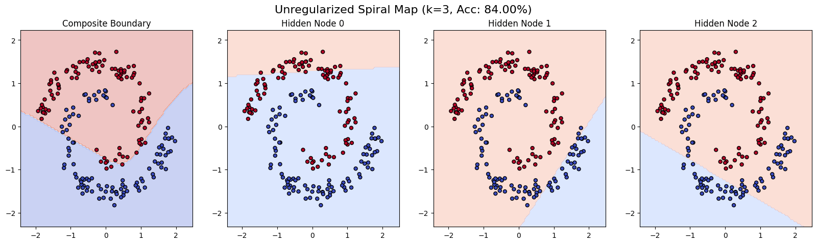
That is the unregularized version. Notice how Hidden Node 1 and Hidden Node 2 carve up the space in similar ways: both are roughly horizontal-ish boundaries through the middle. The composite uses them, but redundantly.

After adding the orthogonality penalty:

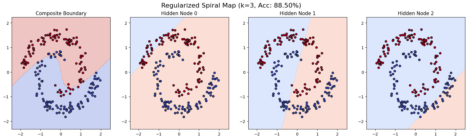
The three nodes have rotated to face different directions. The composite boundary is sharper. Same number of parameters, more useful arrangement.

The order-of-magnitude difference between λ = 1 (broken) and λ = 0.01 (better than baseline) is the lesson worth keeping. Regularization is not a switch. The strength matters more than people give it credit for, and the right strength is dataset-specific. A simpler dataset would tolerate (and benefit from) a heavier penalty. A complex one needs a featherweight.

This generalizes well beyond orthogonality penalties. Weight decay, dropout rate, label smoothing, every regularizer has a sweet spot, and finding it is part of the work, not an afterthought. Papers report the value the authors used. They rarely walk through the failure modes at adjacent values, which is exactly where the intuition lives.

What this whole tinkering taught me

Four experiments. About a weekend of work. Maybe three hundred lines of code. The artifact of value is not the model, which fits on a napkin. It is the set of instincts that came out of running it.

The first instinct is geometric. Hidden-layer width is a function of the dataset’s complexity, not a hyperparameter to be tuned in the abstract. When I look at a new problem now, I find myself asking what shape the decision boundary needs to have, and only then thinking about parameter counts. That is a different starting point than “let me try a few sizes and see.”

The second instinct is about loss functions. Cross-entropy paired with softmax (or sigmoid) is not a stylistic choice. It is the combination where the activation’s derivative cancels out cleanly, leaving a strong gradient signal proportional to the error. MSE on a sigmoid output is the same model, mathematically valid, practically four times slower because of saturation. I had read this rule a dozen times. Now I have watched it.

The third instinct is about how some math is not arbitrary. Softmax-and-cross-entropy collapses to predicted - target. That is a clean, simple thing. Every framework hard-codes them as a single op for that reason. When something in ML feels suspiciously elegant, that is usually the math telling us we are in the right place.

The fourth instinct is that regularization is a continuous dial. Order-of-magnitude differences in λ produce qualitatively different models on the same data. Treating it as on-or-off is leaving a lot on the table.

None of this required fancy infrastructure. All of it required slowing down enough to derive what model.fit() is doing. The specific instincts will keep coming up. The next time someone tells me a model is not converging, I will not ask “what learning rate did you try.” I will ask what loss function and what activation, and whether the gradients are saturating. That is a much better question.