Compressing emojis into 128 numbers, then adding glasses to one

There is a result everyone in deep learning has seen at least once. Take a word embedding model, compute vector("king") - vector("man") + vector("woman"), and the nearest word in the embedding space is queen. The first time we read this it feels like a magic trick. Words have been turned into numbers, the numbers respect human intuition about analogies, and we can do algebra on them.

Then we read about it happening in image space too. There is a famous figure in the original DCGAN paper showing (man with glasses) - (man without glasses) + (woman without glasses) = woman with glasses. Same idea, different modality. I have always nodded along. I have never tested it myself.

So I trained a small convolutional autoencoder on 204 face emojis, encoded them down to 128 numbers each, and then tried to add glasses to one of them by doing arithmetic in the latent space. This post is the writeup.

The actual answer to “does it work” is “kind of, in a way that taught me more than if it had worked perfectly.” The interesting parts are everywhere along the way.

What an autoencoder is, in one paragraph

An autoencoder is a network that learns to copy its input to its output, but with a forced bottleneck in the middle. The encoder squeezes the input into a low-dimensional vector (the latent code, sometimes called z), and the decoder tries to reconstruct the original from that vector alone. If the bottleneck is small enough that the network cannot just memorize, it has to learn something useful: a compressed representation of the data that preserves whatever matters most for reconstruction. The latent space, the territory those compressed vectors live in, is where the interesting questions show up.

Our setup: input is a 64 by 64 RGB image, which is 12,288 numbers. The latent code is 128 numbers. So the bottleneck forces a 96-times compression. Whatever the network keeps in those 128 numbers is its best guess about what an emoji actually is.

The data

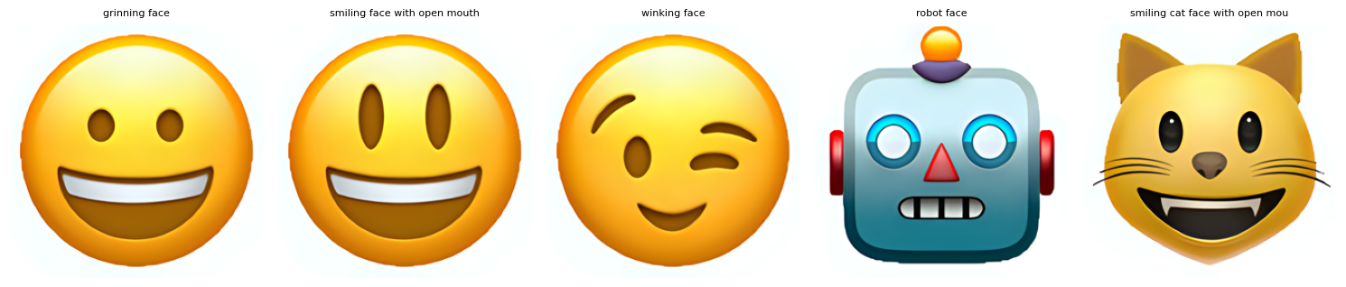
I used the valhalla/emoji-dataset on HuggingFace, which contains 2,749 emojis with text descriptions. To keep things visually consistent, I filtered to the 204 emojis whose description contains the word “face”:

dataset = load_dataset("valhalla/emoji-dataset", split="train")
 
FILTER_KEYWORD = "face"
face_indices = [
    i for i, text in enumerate(dataset['text'])
    if FILTER_KEYWORD.lower() in text.lower()
]
face_dataset = dataset.select(face_indices)
print(f'Emojis containing "{FILTER_KEYWORD}": {len(face_dataset)}')
# Emojis containing "face": 204

Five randomly drawn samples from the filtered set:

204 images is tiny by deep learning standards. Models with millions of parameters tend to memorize that few examples instantly. So I split 60/20/20 (122 train / 40 val / 42 test) and then augmented each split by drawing repeatedly from it with random flips, rotations, color jitter, and small affine transforms, until I had 600 / 200 / 200:

augmentation_transforms = transforms.Compose([
    transforms.RandomHorizontalFlip(p=0.5),
    transforms.RandomRotation(degrees=10),
    transforms.ColorJitter(brightness=0.2, contrast=0.2, saturation=0.2),
    transforms.RandomAffine(degrees=0, translate=(0.05, 0.05), scale=(0.9, 1.1)),
    transforms.Resize((IMG_SIZE, IMG_SIZE)),
])

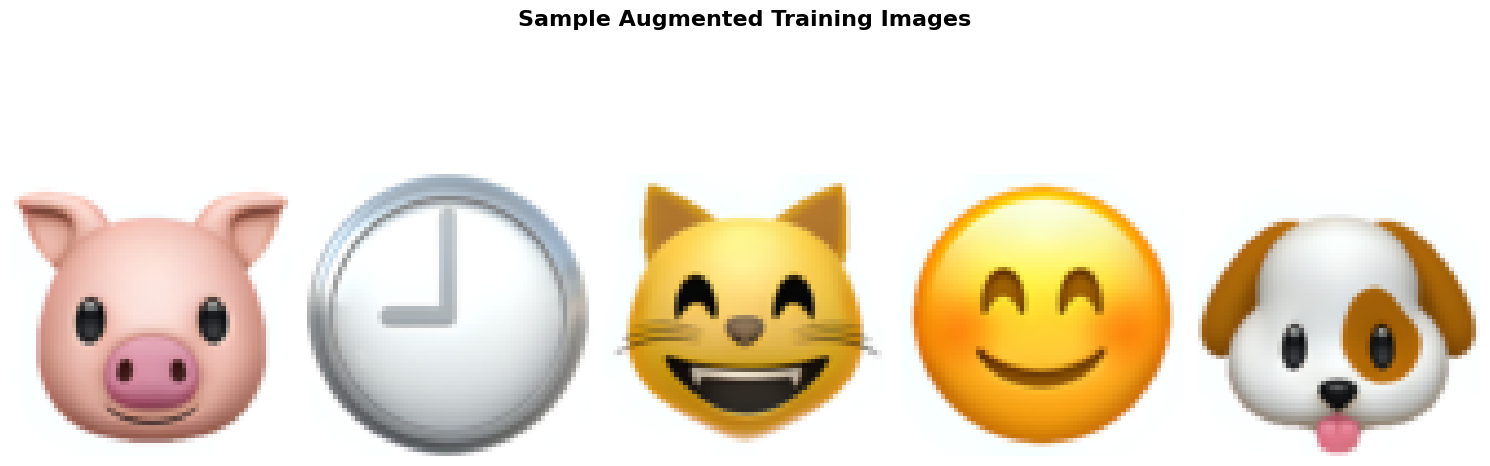
The augmentation is doing a lot of work here. Without it, the model would overfit to 122 training images in the first few epochs. With it, we are essentially asking the network to learn that “an emoji is still the same emoji if it is rotated 8 degrees and shifted 3 pixels,” which is exactly the kind of robustness we want a latent code to encode.

A few of the augmented training samples (some originals, some perturbed copies):

The architecture

The encoder follows a DCGAN-inspired pattern: four strided convolutions that progressively shrink the spatial dimensions while growing the channel count, then a flatten and a fully-connected layer to the 128-dim latent space.

class ConvAutoencoder(nn.Module):
    def __init__(self, latent_dim=128):
        super().__init__()
 
        # Encoder: 3x64x64 -> 32x32x32 -> 64x16x16 -> 128x8x8 -> 256x4x4
        self.enc1 = nn.Sequential(
            nn.Conv2d(3, 32, kernel_size=4, stride=2, padding=1),
            nn.BatchNorm2d(32),
            nn.LeakyReLU(0.2, inplace=True),
        )
        self.enc2 = nn.Sequential(
            nn.Conv2d(32, 64, kernel_size=4, stride=2, padding=1),
            nn.BatchNorm2d(64),
            nn.LeakyReLU(0.2, inplace=True),
        )
        self.enc3 = nn.Sequential(
            nn.Conv2d(64, 128, kernel_size=4, stride=2, padding=1),
            nn.BatchNorm2d(128),
            nn.LeakyReLU(0.2, inplace=True),
        )
        self.enc4 = nn.Sequential(
            nn.Conv2d(128, 256, kernel_size=4, stride=2, padding=1),
            nn.BatchNorm2d(256),
            nn.LeakyReLU(0.2, inplace=True),
        )
        self.encoder_fc = nn.Linear(256 * 4 * 4, latent_dim)
 
        # Decoder: latent -> 256x4x4 -> 128x8x8 -> 64x16x16 -> 32x32x32 -> 3x64x64
        self.decoder_fc = nn.Linear(latent_dim, 256 * 4 * 4)
 
        self.dec1 = nn.Sequential(
            nn.Upsample(scale_factor=2, mode='nearest'),
            nn.Conv2d(256, 128, kernel_size=3, stride=1, padding=1),
            nn.BatchNorm2d(128),
            nn.LeakyReLU(0.2, inplace=True),
        )
        # ... three more upsample-and-conv blocks, mirroring the encoder

A few things in this design are worth slowing down on, because they all encode small lessons.

Strided convolution instead of max pooling. Each Conv2d has stride=2, which halves the spatial dimensions in one operation. Most introductory ML courses teach max pooling for downsampling, but strided convolutions have two advantages here: they are learnable (the network decides how to combine pixels rather than just taking the max), and they preserve gradient information more cleanly during backprop. For autoencoders specifically, where we need to reconstruct fine spatial details on the decoder side, this matters.

Channel growth, spatial shrinkage. As the spatial dimensions go from 64 to 32 to 16 to 8 to 4, the number of channels goes from 3 to 32 to 64 to 128 to 256. The total number of activations at each layer is roughly constant. This is standard practice. Intuitively: as we lose spatial resolution, we need more “feature types” at each location to represent the same information.

LeakyReLU instead of ReLU. Plain ReLU outputs zero for any negative input, which means that any neuron that gets driven into the negative regime stays dead forever (the gradient through the dead neuron is zero, so it cannot recover). LeakyReLU passes a small fraction of the negative signal through (0.2 here), which keeps the gradients alive. For a small network on a small dataset, dead neurons are a real risk, and the asymmetry of LeakyReLU is cheap insurance.

BatchNorm before the activation. BatchNorm rescales the pre-activation outputs to have roughly zero mean and unit variance per channel, which keeps the activations in a regime where the LeakyReLU is meaningful. Without BatchNorm, training a network this deep on a dataset this small is genuinely fragile.

Symmetric decoder using upsample plus conv. The decoder mirrors the encoder, but instead of ConvTranspose2d (which can introduce checkerboard artifacts due to overlapping output strides), I used nearest-neighbor upsampling followed by a regular Conv2d. This is the trick from the Distill article on deconvolution and checkerboard artifacts and it just works.

The full forward pass returns both the reconstruction and the latent code, so we can inspect the latent later:

def forward(self, x):
    z = self.encode(x)
    out = self.decode(z)
    return out, z

Total parameter count: 2,132,515. Most of those are in the two FC layers connecting 256 * 4 * 4 = 4,096 flattened features to and from the 128-dim latent.

Loss: MSE plus a sprinkle of L1

The natural loss for image reconstruction is mean squared error. We want the output pixels to be close to the input pixels, and squaring the difference is the standard way to penalize that.

The problem with MSE alone is that it produces blurry reconstructions. The reason is built into the loss itself. Imagine two equally plausible reconstructions of the same input: one is sharp but slightly off-position, the other is a blurry average of the two possible positions. MSE prefers the average, because squaring the error punishes a sharp wrong answer more than a soft uncertain one. The optimizer learns to hedge.

Adding an L1 (absolute value) term fixes this partially. L1 has no squaring, so it does not over-punish individual pixel mismatches. This biases the model toward sharper reconstructions even when it is uncertain:

mse_criterion = nn.MSELoss()
l1_criterion  = nn.L1Loss()
 
def combined_loss(output, target):
    mse = mse_criterion(output, target)
    l1  = l1_criterion(output, target)
    return mse + (L1_LAMBDA * l1)   # L1_LAMBDA = 0.05

The 0.05 weight is empirical. Too much L1 and the network produces noisy outputs because L1 does not smoothly penalize small differences. Too little and we are back to blurry MSE land. 0.05 was the smallest value where my reconstructions had visible edges.

Training

Adam at lr=1e-3, weight decay 1e-5, batch size 32, max 200 epochs with early stopping at patience 25. ReduceLROnPlateau halves the learning rate when validation loss plateaus for 10 epochs:

optimizer = optim.Adam(model.parameters(), lr=1e-3, weight_decay=1e-5)
scheduler = optim.lr_scheduler.ReduceLROnPlateau(optimizer, mode='min', factor=0.5, patience=10)
 
for epoch in range(1, EPOCHS + 1):
    model.train()
    for batch_x, batch_y in train_loader:
        batch_x, batch_y = batch_x.to(device), batch_y.to(device)
        optimizer.zero_grad()
        output, _ = model(batch_x)
        loss = combined_loss(output, batch_y)
        loss.backward()
        optimizer.step()
 
    # Validation phase
    model.eval()
    with torch.no_grad():
        val_loss = sum(combined_loss(model(x.to(device))[0], y.to(device)).item() * x.size(0)
                       for x, y in val_loader) / len(val_dataset)
 
    scheduler.step(val_loss)
 
    if val_loss < best_val_loss:
        best_val_loss = val_loss
        best_model_state = copy.deepcopy(model.state_dict())
        patience_counter = 0
    else:
        patience_counter += 1
 
    if patience_counter >= PATIENCE:
        print(f"Early stopping at epoch {epoch}. Best val loss: {best_val_loss:.6f}")
        break

Training stopped at epoch 91 with a best validation loss of 0.022369. The learning curves show what is going on:

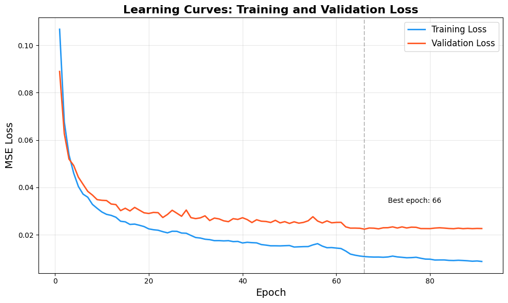
The training loss keeps falling steadily because we are still memorizing more of the training set. The validation loss bottoms out around epoch 80 and starts oscillating, which is the classic shape of “we have learned what generalizes, anything more is overfitting.” Early stopping caught it at the right place. The vertical dashed line marks the best epoch.

Test set MSE was 0.024514, very close to validation loss, which means the model is generalizing and the test set is not unusual relative to validation.

Reconstruction quality

The first thing to check is whether the autoencoder can actually reconstruct an image it has never seen during training. Five randomly drawn input/reconstruction pairs from the test set:

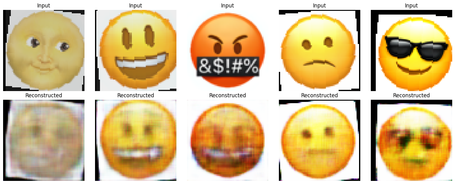
The reconstructions are recognizably the same emojis. The shapes are right, the major colors are right, the eye and mouth positions are mostly right. The reconstructions are also visibly softer than the inputs, with some fine details (eyebrows, exact mouth curvature) blurred out.

This is exactly what we should expect from a 96-times compression with MSE-based loss. The latent code is forced to make tradeoffs, and “exact eyebrow shape” loses to “the shape, color, and position of the face.” The L1 term is helping (the reconstructions are sharper than they would be with MSE alone), but it cannot work miracles. To get sharper reconstructions we would need a larger latent dimension, a deeper decoder, or a fundamentally different loss function (perceptual loss, adversarial loss, or a diffusion-based decoder).

For our actual goal (vector arithmetic), the reconstruction quality is good enough. We need the model to have learned a latent space where similar emojis end up near each other and where moving in particular directions corresponds to changing particular attributes. The blurriness of pixel-level reconstructions does not necessarily indicate that the latent geometry is bad.

The actual interesting part: latent arithmetic

This is the experiment I built the autoencoder for.

The hypothesis is that the latent space the encoder has learned is approximately linear in semantic features. Concretely: if we encode a “nerd face” (which has glasses) and a “smiling face” (which does not), and subtract, what we get should approximately be a “glasses vector” in the 128-dim space. Adding that vector to any other face latent should add glasses to that face when we decode.

glasses_vector  = encode(nerd_face) - encode(smiling_face)
composite_z     = encode(tongue_face) + glasses_vector
composite_image = decode(composite_z)

Whether this works is genuinely uncertain. We did not train the model to support this operation. We trained it to compress and reconstruct. The hope is that good compression and arithmetic-friendly latent geometry come together as a side effect, because both require the same thing: a representation where similar inputs end up near each other and where smooth movements in latent space correspond to smooth changes in the output.

The implementation is just a few lines:

ID_NERD    = 2306   # 'nerd face'
ID_SMILE   = 1      # 'smiling face with open mouth'
ID_TONGUE  = 1335   # 'face with tongue'
 
model.eval()
with torch.no_grad():
    z_nerd   = model.encode(get_emoji_by_idx(ID_NERD).unsqueeze(0))
    z_smile  = model.encode(get_emoji_by_idx(ID_SMILE).unsqueeze(0))
    z_target = model.encode(get_emoji_by_idx(ID_TONGUE).unsqueeze(0))
 
    # Target + (Nerd - Smile)
    z_composite     = z_target + (z_nerd - z_smile)
    composite_image = model.decode(z_composite).cpu().squeeze(0)

And the result:

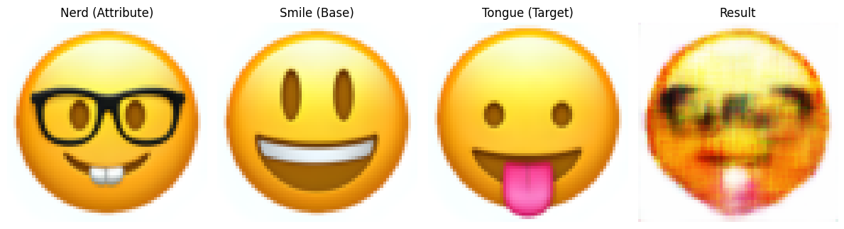
The composite has the overall shape and color of the target (tongue face), but the eye region has changed in a direction that matches the glasses attribute. There is a clear darkening and structural shift around the eyes that is not present in the original tongue face. The mouth and tongue are largely preserved.

Did it succeed? Partially. We can definitely see that the latent direction z_nerd - z_smile encodes something about the eyes, because adding it to a different face changes the eye region. But the result is not as crisp as the analogous figure in the DCGAN paper. The glasses are suggested rather than drawn. The composite reads as “tongue face with vague glasses-ish modification around the eyes.”

The reasons it is not crisper are interesting on their own:

1. The latent space is not perfectly linear. A vanilla autoencoder has no incentive to make its latent space arithmetic-friendly. It just wants reconstructions to be good. The latent space ends up roughly arrangement-friendly because of how the network learns, but not perfectly. Variational autoencoders (VAEs) explicitly enforce a Gaussian prior on the latent distribution, which makes the space much more linear and dramatically improves arithmetic. We did not use a VAE.

2. 128 dimensions is small for this kind of operation. Word2vec uses 300 to 1,000 dimensions for words. DCGAN uses 100 to 200 for images. We picked 128 to enforce strong compression. The cost is that semantic features are tangled together (one dimension might encode “eye darkness” but also partially encode “head tilt”), so isolating one specific attribute (glasses) by subtracting two examples is going to be noisy.

3. Two examples is not enough to define an attribute direction reliably. A more robust approach would average over many (with-glasses, without-glasses) pairs to get a cleaner glasses vector. With one pair, we are getting “the difference between these two specific faces, which happens to include glasses but also includes everything else that differs between them.”

So the result is a partial confirmation. The latent space supports arithmetic, but with limitations that match what the theory would predict.

Three instincts that came out of this

The first instinct is about why convolutional architectures are the right shape for image autoencoders. The strided downsampling preserves spatial structure, the channel growth compensates for resolution loss, and the symmetric decoder lets us reconstruct without losing the inductive bias that pixels near each other are related. None of this is novel. All of it was abstract until I built it.

The second instinct is that the choice of loss has visible signatures. MSE alone produces blurry output because it rewards averaging when the model is uncertain. Adding L1 sharpens reconstructions because L1 does not over-punish single-pixel errors. These are not abstract claims, they are predictions we can verify by toggling the loss and looking at the output. Most ML papers do not have time to walk through this. The experiment takes ten minutes.

The third instinct is the most useful one. The fact that vector arithmetic on the latent space partially works tells us something about what the autoencoder actually learned. It learned a representation where similar emojis end up near each other and where small movements in latent space correspond to small semantic changes. That is a non-trivial property, and it is the property that makes the entire pre-trained-embeddings ecosystem work, from word2vec to CLIP to modern diffusion model conditioning. Anywhere a model takes an embedding as input, the assumption is that the embedding space has this kind of structure. The emoji experiment is a tiny version of the same question that anyone working with embeddings runs into eventually: does this representation actually support the operations I want to do on it? The way to find out is to test.