A tiny pre-trained transformer was sitting on my disk. It had been trained on synthetic math problems with a very specific structure: each problem was 20 tokens long, with variable assignments, an operator, and an answer position the model needed to predict. Most of the time it nailed the answer. Sometimes it embarrassed itself.
The same model was getting 66 percent correct-answer probability on some a * a problems and 4.6 percent on others. Same operator. Same input format. Same weights. Why the spread?
To find out, I rewrote the model’s attention mechanism in pure Python (no torch.matmul, no vectorization, just nested for-loops), captured the 20-by-20 attention matrix on the way through, plotted heatmaps for the cases the model was getting right versus wrong, and then went one step further: I surgically intervened on specific cells of that matrix to force the model to look at the right tokens. Without retraining anything, I lifted the bad-example accuracy from 4.65 percent to 32.52 percent.
This post walks through that experiment. It is the most interesting thing I have built so far, partly because it is a tiny version of the kind of mechanistic interpretability work that labs like Anthropic and DeepMind are doing on frontier models, and partly because the result is fun: attention is a real thing we can inspect, plot, and edit.
The system under inspection
The pre-trained model was a small decoder-only transformer (GPT-style): 6 layers, 8 attention heads, d_model=512, vocabulary made of digits and a handful of structural tokens. The job was to predict the answer in math problems formatted like this:
position:  0       1  2  3  4  5  6  7  8  9      10 11 12   13  14 15 16 17 18    19
token:     [START] a  5  b  3  c  7  d  2  [VARS] a  c  [EQ] ans =  a  *  c  [ANS] ?
The first nine positions set up four variable assignments. Position 9 is a [VARS] separator. Positions 10 and 11 list which two variables the equation uses. Positions 12 to 17 spell out the equation in a fixed format (ans = lhs op rhs), and position 19 is the answer the model is supposed to fill in. The format is deliberately rigid so we can interpret what is happening.
For a problem like a = 5, c = 7, ans = a * c, the right answer at position 19 is 35. The model emits a probability distribution over the vocabulary, and the question is whether the highest probability lands on 35.
Some of these the model could solve. Some it could not. I wanted to know what was going on inside its head when it failed.
What attention actually does, in one paragraph
Self-attention is a mechanism that lets every token in a sequence look at every other token and decide how much to weight each one. For each token at position i, the network produces three vectors: a query qᵢ, a key kᵢ, and a value vᵢ. To compute the new representation for position i, we compare qᵢ to every other token’s key by dot product, normalize the resulting scores into a probability distribution with softmax, and then take a weighted average of the value vectors:
attention_score(i, j) = (qᵢ · kⱼ) / sqrt(d_k)
weight(i, j) = softmax over j of attention_score(i, j)
output(i) = Σⱼ weight(i, j) · vⱼ
The intuition: each query is asking “what other positions are relevant to me right now?” The keys answer “here is what I have to offer.” The values are the actual content that gets pulled forward. The whole transformer is just stacks of this, plus position information and feedforward layers.
For our math model, the most important query is the one emitted at position 18 (the [ANS] token). It is essentially asking the rest of the sequence: “I am about to predict the final answer. What do I need to look at?” The pattern of weights it produces is what we want to inspect.
Rewriting attention in for-loops
The standard implementation of attention is one line of vectorized code: scores = (Q @ K.T) / sqrt(d_k); weights = softmax(scores); out = weights @ V. Fast. Opaque.
For debugging, I needed something I could intercept at every step. So I rewrote the entire attention function as four nested for-loops. This is laughably slow (it would be a felony to ship this to production), but it lets us capture the exact 20-by-20 probability matrix and inspect it later:
def attention(q, k, v, d_k, mask=None):
    seq_len = 20
    scale = math.sqrt(d_k)

    q_list = q.tolist()
    k_list = k.tolist()
    v_list = v.tolist()

    # Step 1: dot product Q · K^T, scaled
    raw_scores = np.zeros((1, 1, seq_len, seq_len), np.float32)
    for i in range(seq_len):
        for j in range(seq_len):
            dot = 0.0
            for kk in range(d_k):
                dot += q_list[0][0][i][kk] * k_list[0][0][j][kk]
            raw_scores[0][0][i][j] = dot / scale

    # Step 2: causal mask (future tokens are -infinity)
    if mask is not None:
        mask_list = mask.tolist()
        for i in range(seq_len):
            for j in range(seq_len):
                if mask_list[0][i][j] == 0:
                    raw_scores[0][0][i][j] = -1e9

    # Step 3: numerically stable softmax, row by row
    prob_scores = np.zeros((1, 1, seq_len, seq_len), np.float32)
    for i in range(seq_len):
        row_max = max(raw_scores[0][0][i][j] for j in range(seq_len))
        row_sum = 0.0
        for j in range(seq_len):
            prob_scores[0][0][i][j] = math.exp(raw_scores[0][0][i][j] - row_max)
            row_sum += prob_scores[0][0][i][j]
        for j in range(seq_len):
            prob_scores[0][0][i][j] /= row_sum

    # Step 4: weighted sum of values
    out = np.zeros((1, 1, seq_len, d_k), np.float32)
    for i in range(seq_len):
        for kk in range(d_k):
            val = 0.0
            for j in range(seq_len):
                val += prob_scores[0][0][i][j] * v_list[0][0][j][kk]
            out[0][0][i][kk] = val

    # Capture the probability matrix in a global so we can plot it later
    global global_attention_scores
    global_attention_scores = prob_scores[0][0].copy()

    return torch.from_numpy(out).to(q.device)
To verify the rewrite was equivalent to PyTorch’s vectorized version, I saved the captured 20-by-20 attention matrix from one specific test example (observation 1979) into a CSV, then ran the same example through the for-loop version and compared:
def validate_attention_csv(scores_2d, output_2d, obs_id, d_k):
    # Compare element-by-element against the saved reference
    with open(f'{obs_id}_scores_{d_k}.csv') as f:
        max_diff = 0.0
        for i, row in enumerate(csv.reader(f)):
            for j, val in enumerate(row):
                if val.strip():
                    diff = abs(float(val) - scores_2d[i][j])
                    max_diff = max(max_diff, diff)
        print(f"Max diff: {max_diff:.6f}  {'PASS' if max_diff < 0.001 else 'FAIL'}")
Max difference: under 1e-6. The for-loops produced the same numbers as PyTorch.
The only purpose of this exercise was to give us a hook. With the global capture in place, every forward pass leaves a record of the full attention pattern. Now we can ask the model to solve a problem, watch where it looked, and figure out what went wrong when it failed.
What attention looks like when the model gets it right
I pulled 10 examples from the test set where the model was confident in the right answer (average correct-answer probability: 66 percent), ran each through the model, and averaged the captured attention matrices. The result is an attention heatmap where the row is the query position, the column is the key position, and the brightness is the weight assigned:
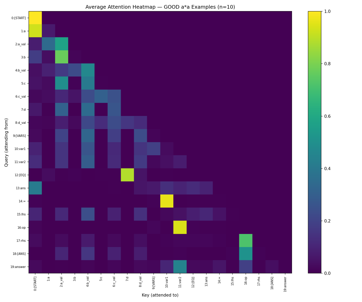
A few patterns are obvious even at a glance.
The diagonal-ish band on the upper-left is the attention pattern for variable definition tokens, which mostly attend to themselves and the variable name immediately preceding them. This makes sense: positions 1 to 8 are setting up a=5, b=3, c=7, d=2, and each value position pays attention to its own variable name.
Position 12 (the [EQ] separator) attends strongly to position 7 (the variable d), which is a slight oddity but not the failure mode.
Position 14 (the = sign) attends strongly to position 10 (var1), which is exactly right: when we hit the equals sign, we are about to spell out which variables get used.
Position 16 (the operator) attends strongly to position 11 (var2).
The interesting row is row 18, the [ANS] query. This is the token whose attention pattern most directly determines the answer the model produces. In the good heatmap, row 18 places strong weight on position 16 (the * operator, around 51 percent) and meaningful additional weight on position 2 (the value of variable a, around 11 percent). The model is essentially saying: “I am about to answer. The operator is multiplication. The relevant value is a_val.” Which is exactly what we would want it to do for an a * a problem.
What attention looks like when the model fails
I did the same averaging for 12 test examples where the model was getting the wrong answer (average correct-answer probability: 4.6 percent):

Side by side, the broad structure looks almost identical. The model has learned the format. The diagonal patterns are there. Position 14 still attends to var1. Position 16 still attends to var2. Row 18 still puts most of its weight on the operator at position 16, also around 51 percent.
The difference is in how the rest of row 18 is distributed across the value positions.
In the good subset, row 18 puts about 11 percent on position 2 (a_val). Reasonable, given these are a * a problems and the operand value is what the model needs.
In the bad subset, that 11 percent shifts. Position 2 gets less weight. Position 6 (c_val) and position 8 (d_val) each pick up an extra few percentage points. The model is attending to the wrong numbers. It still knows the operator is multiplication. It is just multiplying with the wrong values.
This tells us something important about the failure mode. The model is not failing at understanding the operator, or the format, or what an answer position is. It is failing at variable binding: matching the variable names in the equation (lhs and rhs at positions 15 and 17) to their values earlier in the sequence. When variable binding goes wrong, the model still confidently predicts an answer. It just predicts the wrong answer, with the same operator applied to the wrong operands.
This is a meaningful insight on its own. Most “the transformer made a mistake” stories assume the failure is at some fuzzy level of reasoning. Here, the failure is at a very specific, very localized step: looking up the right number to plug into a known operator. Knowing this, we can do something about it.
Surgically fixing the model without retraining
If the failure is variable-binding, we should be able to fix it without changing any model weights. We just need to nudge attention back toward the correct value positions when we know the model is about to produce an answer.
The plan: when the attention function is called and we are computing row 18 (the [ANS] query), look at the current sequence to figure out which variables are being referenced (positions 15 and 17 hold the variable names), find which of the value positions (2, 4, 6, 8) hold their values, and add a small positive constant to those raw scores before softmax. Same for the operator position at 16, which we want to keep prominent.
# Question 3: Manual attention boost (before softmax)
if adjust_attention and CURRENT_TRG is not None:
    lhs_var = CURRENT_TRG[0, 15].item()  # variable name at lhs
    rhs_var = CURRENT_TRG[0, 17].item()  # variable name at rhs

    # Variable definition pairs: (var_name_pos, value_pos)
    for var_idx, val_pos in [(1, 2), (3, 4), (5, 6), (7, 8)]:
        var_name = CURRENT_TRG[0, var_idx].item()
        if var_name == lhs_var or var_name == rhs_var:
            raw_scores[0][0][18][val_pos] += boost_amount   # +2.0

    # Also boost the operator position
    raw_scores[0][0][18][16] += boost_amount
That is the entire intervention. We are not retraining. We are not even touching weights. We are reaching into a single forward pass and adding a constant of +2.0 to a small number of pre-softmax raw scores.
The reason we apply the boost before softmax is important. After softmax, the row is a probability distribution that sums to 1, and adding to it would break that. Before softmax, we are working with raw logits, and adding a constant just shifts the relative magnitude. The softmax will still produce a valid distribution; that distribution will just put more mass on the boosted positions.
I re-ran the same 12 bad examples with the intervention turned on. The accuracy went from 4.65 percent to 32.52 percent on average. A 7x improvement, with no retraining and zero gradient updates.
The improved attention heatmap shows what changed:
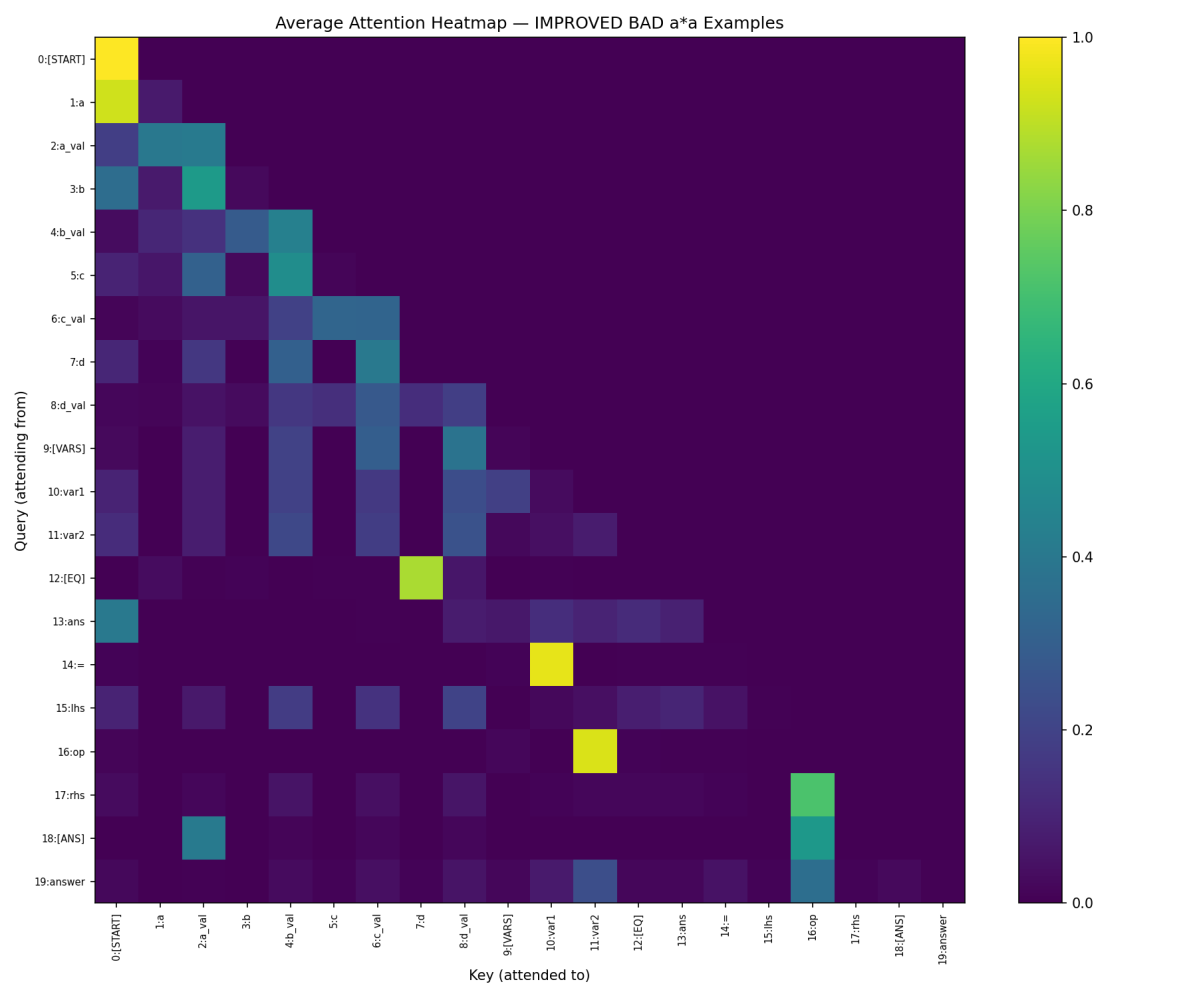
Look at row 18. Position 2 (a_val) is now noticeably brighter than it was in the unintervened bad heatmap. The model is now attending to the correct operand value, and that single change shifts the answer probability dramatically.
Some examples improved by 60 percentage points or more after the intervention. A few got worse. The improvement is not universally robust, which makes sense: the boost amount is fixed at 2.0, but the natural raw-score scale varies across examples. A boost that is the right size for one problem may be too aggressive or too weak for another. With more careful per-example calibration, the gains would be larger and more consistent.
What this whole thing taught me
The first instinct that came out of this is that attention is genuinely interpretable. It is not a black box. The 20-by-20 matrix is right there. We can save it to a CSV, plot it as a heatmap, average it across examples, and see exactly which positions a query is consulting at any layer of the model. The reason this gets framed as some advanced research technique in mechanistic interpretability is because doing it cleanly on a 175-billion-parameter model with thousands of attention heads is hard. Doing it on a small model with 8 heads is doable in an afternoon.
The second instinct is that transformer failures are often retrieval failures rather than reasoning failures. The model in this experiment understood multiplication. It knew the format. It correctly identified that it was supposed to predict an answer. It just grabbed the wrong number from earlier in the sequence. This kind of failure mode has been studied at scale (it underlies a lot of work on “bound variable” failures in larger LMs), and it shows up at every model size.
The third instinct is that we have more levers than just retraining. Activation patching, attention masking, steering vectors, residual stream interventions are all real tools that people use to change model behavior without changing weights. The intervention in this experiment is the simplest possible version of that idea: add a constant to a few pre-softmax scores. The fact that this works at all is what makes the broader research direction interesting.
The fourth instinct is more subjective. Spending an afternoon writing attention in for-loops, then looking at the heatmaps, then surgically intervening on the model is the most viscerally satisfying thing I have done in deep learning. The system is small enough that we can hold all of it in our head, and the experiments are conclusive enough that we can actually answer the question we set out to ask. Most ML research at the frontier is the opposite of this: huge models, fuzzy results, compute-bound iterations. The small system is where understanding happens. It is worth coming back to it deliberately, even when we have access to better infrastructure.